
Parameters as a System: How Lending-Protocol Risk Parameters Emerge from a Single Pipeline
Risk parameters in lending protocols are conventionally set in sequence. A loan-to-value ratio is anchored on the asset's volatility profile. A liquidation bonus is calibrated by reference to peer protocols. Supply and borrow caps are set against circulating supply or recent on-chain volume. Interest-rate parameters are usually drawn from a template. Each of these choices has a clear local rationale. What happens when those locally-rational choices fail together is the subject of a companion piece reviewing six stress events from 2022 to 2025.
The framework presented in this series treats parameter setting as a single system rather than a collection of independent calibrations. Seven steps run in a deliberate order: a qualitative gate that decides whether quantitative work proceeds at all, an asset-level analysis that establishes what the asset can bear on its own terms, a protocol-level analysis that adjusts those findings against the liquidation machinery actually in place, and a validation layer that tests the resulting configuration against history and against futures that have not yet happened. Each step consumes the output of the previous one. No parameter is final until the whole pipeline has run.
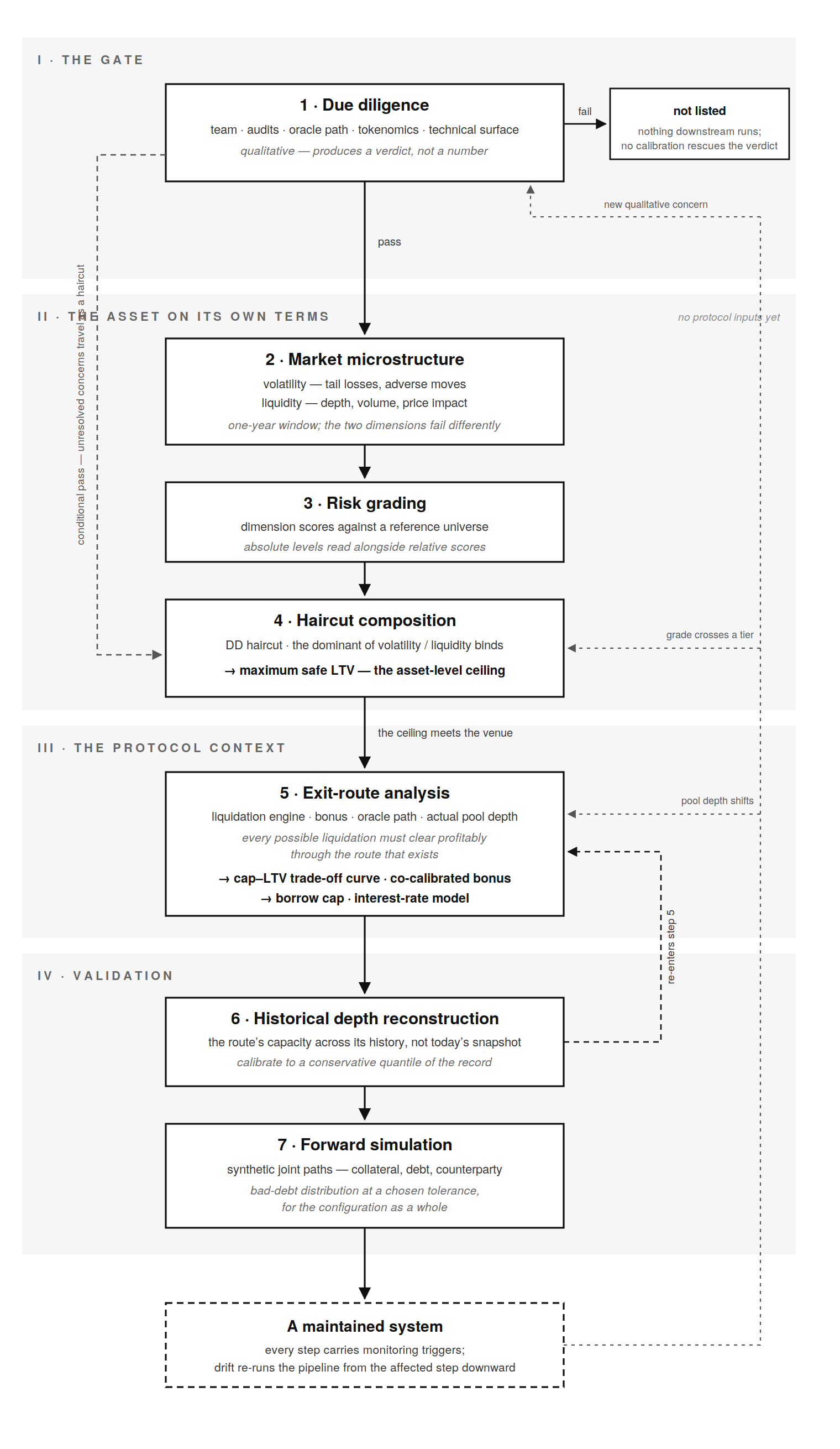
This post lays out that logic in general terms: what each stage does, why it sits where it sits, and what passes from one to the next. The posts that follow develop each step in depth.
The gate: Due Diligence decides whether anything else run
The pipeline opens with a step that produces no numbers at all. Due Diligence is a qualitative review of the asset's fundamentals: the team behind it, the audit record, the oracle architecture through which the protocol will price it, the tokenomics, and the technical surface of the token contract itself.
Its output is a gate. An asset that fails does not proceed to calibration, since there is no volatility profile favourable enough, and no cap conservative enough to compensate for an unauditable contract or an oracle path that can be manipulated or any other serious quality concerns. Quantitative analysis answers the question of how much exposure is tolerable; it cannot answer whether exposure should exist at all. That question is answered here, once, before any market data is pulled.
An asset that passes conditionally proceeds, but not cleanly. Each unresolved structural concern identified in the review is carried forward as a discretionary haircut that will tighten the parameters produced downstream. The gate, in other words, does not merely open or close; when it opens partially, the width of the opening travels with the asset through the rest of the pipeline.
The asset on its own terms
The next three steps characterise the asset independently of any protocol that might list it.
First, market microstructure. The asset's behaviour over the preceding year is summarised across two dimensions: volatility — how large its adverse moves are, and how heavy its tails. And liquidity — how much depth stands behind its price, how its volume has trended, and how much a dollar of trading moves the market. The two dimensions are kept separate deliberately, because they fail differently: volatility determines how quickly a position can breach its threshold, while liquidity determines what it costs to exit once it does.
Second, risk grading. The raw measurements are placed against a reference universe of the broader market, producing a score for each dimension and a composite. The relative framing is informative but is not allowed to launder risk: an asset can grade moderately against a universe that includes extreme instruments while remaining extreme in absolute terms, and the framework reads both the relative score and the absolute level.
Third, the initial parameter recommendation. The dimension grades and the concerns carried forward from due diligence are composed into haircuts against the protocol's reference ceiling, producing a maximum safe loan-to-value (LTV) ratio. Volatility and liquidity protect against the same failure (a liquidation that arrives too late or costs too much), so their haircuts do not stack; the dominant risk dimension binds. The result is a ceiling derived entirely from what the asset is. It does not yet know anything about pool depth, borrower demand, or the protocol's liquidation engine, and that is by construction: it is the level above which the asset should not be leveraged anywhere, under any market structure.
The protocol context: parameters meet the actual liquidation path
The asset-level ceiling is a boundary, not a recommendation. The next step adjusts the parameters against the machinery that will actually enforce them: the protocol's liquidation engine, its close factor and bonus, its oracle configuration, and most consequentially, the exit route through which seized collateral will actually be sold.
The governing requirement is straightforward to state: every liquidation the parameter set can produce must be executable at a profit through the route that exists, not the route one would wish for. The route has finite depth, and selling into it moves the price; beyond a certain size, the cost of exit exceeds the liquidator's bonus, no rational liquidator acts, and the position degrades into bad debt while remaining nominally liquidatable. The largest position the protocol can genuinely unwind is a property of the pool, not of the liquidation logic.
Holding parameters to this requirement couples them. The supply cap determines how large a liquidation can arrive; the loan-to-value ratio determines how much debt stands behind a given amount of collateral; the bonus determines the budget available to absorb exit costs; and the pool's depth determines what that budget can buy. Rather than resolving this into a single recommended number, the framework produces the trade-off itself: a curve of internally consistent cap-and-LTV combinations, each safe with respect to the exit route, along which a higher ratio is available at the price of a tighter cap. Governance chooses the operating point according to its growth-versus-risk preference, with the assurance that every point on the curve respects the constraint. The debt-side parameters (the borrow cap and the interest-rate curve) are calibrated in the same pass, sized so that the rate mechanism remains active across the realistic demand range rather than becoming decorative.
Validation: against the past, and against futures not yet realised
The first five steps produce a calibration against the current state of the world. The last two test whether that calibration deserves confidence.
The first validation looks backward. Today's pool depth is one draw from a distribution, and often a favourable one. The framework reconstructs the exit route's capacity across its history and calibrates against a conservative quantile of that record rather than the present snapshot. Where today's depth is the high-water mark, this materially tightens the recommended configuration.
The second validation looks forward. Synthetic joint price paths are generated for the collateral, the debt asset, and the pool's counterparty asset preserving volatility clustering and tail dependence, and the chosen parameter set is run against thousands of them. The output is a distribution of bad-debt outcomes for the configuration as a whole, and a probabilistic statement at a chosen tolerance, rather than an assurance derived from any single scenario.
A maintained system, not a report
Because every step consumes the outputs of the steps before it, a change in any input has a defined blast radius. Each step therefore carries explicit monitoring triggers that re-run the pipeline from the affected point downward: a structural shift in pool depth re-runs the protocol-level calibration; a grade crossing a tier boundary re-runs the haircut composition; a newly surfaced qualitative concern returns the asset to the gate itself. The framework's output is not a parameter set at a moment in time but the trajectory of parameters under change which is what a lending protocol actually operates.
What follows
The posts in this series develop the individual steps in depth: the due-diligence methodology and its gating logic, the market-microstructure characterisation and grading algorithm, the haircut composition behind the asset-level ceiling, the exit-route analysis and the cap–LTV trade-off surface it produces, the historical depth reconstruction, and the simulation methodology along with the framework's extensions across protocol architectures from isolated markets to curator vaults. The pieces are connected; the order in which they are read is not.